音频特征提取

torchaudio 实现了音频领域常用的特征提取方法。它们在 torchaudio.functional 和 torchaudio.transforms 中可用。

functional 以独立函数的形式实现功能。 它们是无状态的。

transforms 将功能实现为对象， 使用来自 functional 和 torch.nn.Module 的实现。由于所有 转换都是 torch.nn.Module 的子类，它们可以使用 TorchScript 进行序列化。

有关可用功能的完整列表，请参阅文档。在本教程中，我们将探讨时域和频域之间的转换 (Spectrogram, GriffinLim, MelSpectrogram)。

# When running this tutorial in Google Colab, install the required packages
# with the following.
# !pip install torchaudio librosa

import torch
import torchaudio
import torchaudio.functional as F
import torchaudio.transforms as T

print(torch.__version__)
print(torchaudio.__version__)

Out:

1.10.0+cpu
0.10.0+cpu

准备数据和实用函数（跳过此部分）

#@title Prepare data and utility functions. {display-mode: "form"}
#@markdown
#@markdown You do not need to look into this cell.
#@markdown Just execute once and you are good to go.
#@markdown
#@markdown In this tutorial, we will use a speech data from [VOiCES dataset](https://iqtlabs.github.io/voices/), which is licensed under Creative Commos BY 4.0.

#-------------------------------------------------------------------------------
# Preparation of data and helper functions.
#-------------------------------------------------------------------------------

import os
import requests

import librosa
import matplotlib.pyplot as plt
from IPython.display import Audio, display


_SAMPLE_DIR = "_assets"

SAMPLE_WAV_SPEECH_URL = "https://pytorch-tutorial-assets.s3.amazonaws.com/VOiCES_devkit/source-16k/train/sp0307/Lab41-SRI-VOiCES-src-sp0307-ch127535-sg0042.wav"
SAMPLE_WAV_SPEECH_PATH = os.path.join(_SAMPLE_DIR, "speech.wav")

os.makedirs(_SAMPLE_DIR, exist_ok=True)


def _fetch_data():
  uri = [
    (SAMPLE_WAV_SPEECH_URL, SAMPLE_WAV_SPEECH_PATH),
  ]
  for url, path in uri:
    with open(path, 'wb') as file_:
      file_.write(requests.get(url).content)

_fetch_data()

def _get_sample(path, resample=None):
  effects = [
    ["remix", "1"]
  ]
  if resample:
    effects.extend([
      ["lowpass", f"{resample // 2}"],
      ["rate", f'{resample}'],
    ])
  return torchaudio.sox_effects.apply_effects_file(path, effects=effects)

def get_speech_sample(*, resample=None):
  return _get_sample(SAMPLE_WAV_SPEECH_PATH, resample=resample)

def print_stats(waveform, sample_rate=None, src=None):
  if src:
    print("-" * 10)
    print("Source:", src)
    print("-" * 10)
  if sample_rate:
    print("Sample Rate:", sample_rate)
  print("Shape:", tuple(waveform.shape))
  print("Dtype:", waveform.dtype)
  print(f" - Max:     {waveform.max().item():6.3f}")
  print(f" - Min:     {waveform.min().item():6.3f}")
  print(f" - Mean:    {waveform.mean().item():6.3f}")
  print(f" - Std Dev: {waveform.std().item():6.3f}")
  print()
  print(waveform)
  print()

def plot_spectrogram(spec, title=None, ylabel='freq_bin', aspect='auto', xmax=None):
  fig, axs = plt.subplots(1, 1)
  axs.set_title(title or 'Spectrogram (db)')
  axs.set_ylabel(ylabel)
  axs.set_xlabel('frame')
  im = axs.imshow(librosa.power_to_db(spec), origin='lower', aspect=aspect)
  if xmax:
    axs.set_xlim((0, xmax))
  fig.colorbar(im, ax=axs)
  plt.show(block=False)

def plot_waveform(waveform, sample_rate, title="Waveform", xlim=None, ylim=None):
  waveform = waveform.numpy()

  num_channels, num_frames = waveform.shape
  time_axis = torch.arange(0, num_frames) / sample_rate

  figure, axes = plt.subplots(num_channels, 1)
  if num_channels == 1:
    axes = [axes]
  for c in range(num_channels):
    axes[c].plot(time_axis, waveform[c], linewidth=1)
    axes[c].grid(True)
    if num_channels > 1:
      axes[c].set_ylabel(f'Channel {c+1}')
    if xlim:
      axes[c].set_xlim(xlim)
    if ylim:
      axes[c].set_ylim(ylim)
  figure.suptitle(title)
  plt.show(block=False)

def play_audio(waveform, sample_rate):
  waveform = waveform.numpy()

  num_channels, num_frames = waveform.shape
  if num_channels == 1:
    display(Audio(waveform[0], rate=sample_rate))
  elif num_channels == 2:
    display(Audio((waveform[0], waveform[1]), rate=sample_rate))
  else:
    raise ValueError("Waveform with more than 2 channels are not supported.")

def plot_mel_fbank(fbank, title=None):
  fig, axs = plt.subplots(1, 1)
  axs.set_title(title or 'Filter bank')
  axs.imshow(fbank, aspect='auto')
  axs.set_ylabel('frequency bin')
  axs.set_xlabel('mel bin')
  plt.show(block=False)

def plot_pitch(waveform, sample_rate, pitch):
  figure, axis = plt.subplots(1, 1)
  axis.set_title("Pitch Feature")
  axis.grid(True)

  end_time = waveform.shape[1] / sample_rate
  time_axis = torch.linspace(0, end_time,  waveform.shape[1])
  axis.plot(time_axis, waveform[0], linewidth=1, color='gray', alpha=0.3)

  axis2 = axis.twinx()
  time_axis = torch.linspace(0, end_time, pitch.shape[1])
  ln2 = axis2.plot(
      time_axis, pitch[0], linewidth=2, label='Pitch', color='green')

  axis2.legend(loc=0)
  plt.show(block=False)

def plot_kaldi_pitch(waveform, sample_rate, pitch, nfcc):
  figure, axis = plt.subplots(1, 1)
  axis.set_title("Kaldi Pitch Feature")
  axis.grid(True)

  end_time = waveform.shape[1] / sample_rate
  time_axis = torch.linspace(0, end_time,  waveform.shape[1])
  axis.plot(time_axis, waveform[0], linewidth=1, color='gray', alpha=0.3)

  time_axis = torch.linspace(0, end_time, pitch.shape[1])
  ln1 = axis.plot(time_axis, pitch[0], linewidth=2, label='Pitch', color='green')
  axis.set_ylim((-1.3, 1.3))

  axis2 = axis.twinx()
  time_axis = torch.linspace(0, end_time, nfcc.shape[1])
  ln2 = axis2.plot(
      time_axis, nfcc[0], linewidth=2, label='NFCC', color='blue', linestyle='--')

  lns = ln1 + ln2
  labels = [l.get_label() for l in lns]
  axis.legend(lns, labels, loc=0)
  plt.show(block=False)

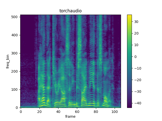
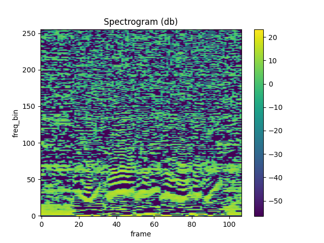
频谱图

要获取音频信号随时间变化的频率构成， 您可以使用 Spectrogram。

waveform, sample_rate = get_speech_sample()

n_fft = 1024
win_length = None
hop_length = 512

# define transformation
spectrogram = T.Spectrogram(
    n_fft=n_fft,
    win_length=win_length,
    hop_length=hop_length,
    center=True,
    pad_mode="reflect",
    power=2.0,
)
# Perform transformation
spec = spectrogram(waveform)

print_stats(spec)
plot_spectrogram(spec[0], title='torchaudio')

Out:

Shape: (1, 513, 107)
Dtype: torch.float32
 - Max:     4000.533
 - Min:      0.000
 - Mean:     5.726
 - Std Dev: 70.301

tensor([[[7.8743e+00, 4.4462e+00, 5.6781e-01,  ..., 2.7694e+01,
          8.9546e+00, 4.1289e+00],
         [7.1094e+00, 3.2595e+00, 7.3520e-01,  ..., 1.7141e+01,
          4.4812e+00, 8.0840e-01],
         [3.8374e+00, 8.2490e-01, 3.0779e-01,  ..., 1.8502e+00,
          1.1777e-01, 1.2369e-01],
         ...,
         [3.4699e-07, 1.0605e-05, 1.2395e-05,  ..., 7.4096e-06,
          8.2065e-07, 1.0176e-05],
         [4.7173e-05, 4.4330e-07, 3.9445e-05,  ..., 3.0623e-05,
          3.9746e-07, 8.1572e-06],
         [1.3221e-04, 1.6440e-05, 7.2536e-05,  ..., 5.4662e-05,
          1.1663e-05, 2.5758e-06]]])

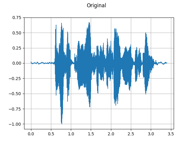
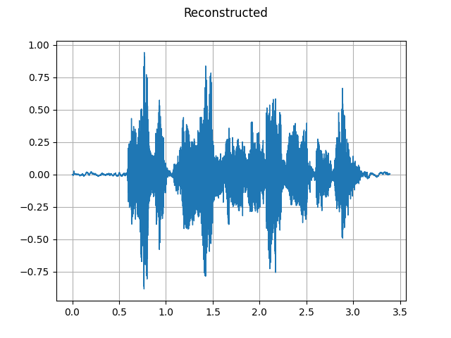
GriffinLim

要从频谱图恢复波形，您可以使用 GriffinLim。

torch.random.manual_seed(0)
waveform, sample_rate = get_speech_sample()
plot_waveform(waveform, sample_rate, title="Original")
play_audio(waveform, sample_rate)

n_fft = 1024
win_length = None
hop_length = 512

spec = T.Spectrogram(
    n_fft=n_fft,
    win_length=win_length,
    hop_length=hop_length,
)(waveform)

griffin_lim = T.GriffinLim(
    n_fft=n_fft,
    win_length=win_length,
    hop_length=hop_length,
)
waveform = griffin_lim(spec)

plot_waveform(waveform, sample_rate, title="Reconstructed")
play_audio(waveform, sample_rate)

• 
• 

Out:

<IPython.lib.display.Audio object>
<IPython.lib.display.Audio object>

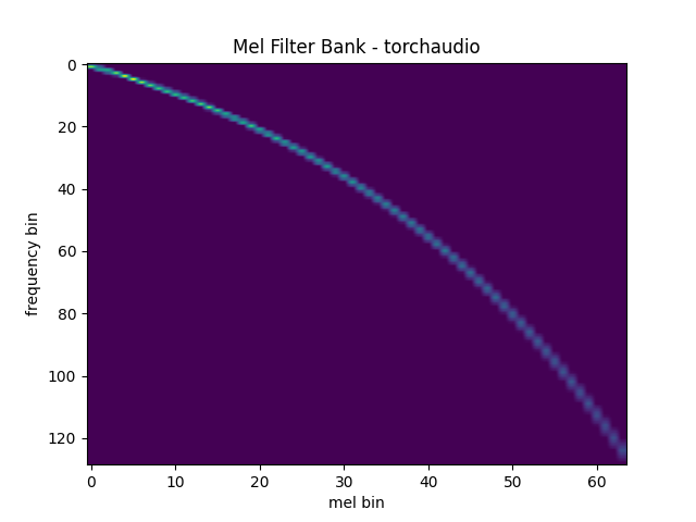
梅尔滤波器组

torchaudio.functional.create_fb_matrix 生成滤波器组，用于将频率 bin 转换为 mel 刻度 bin。

由于此函数不需要输入音频/特征，因此在 torchaudio.transforms 中没有等效的转换。

n_fft = 256
n_mels = 64
sample_rate = 6000

mel_filters = F.create_fb_matrix(
    int(n_fft // 2 + 1),
    n_mels=n_mels,
    f_min=0.,
    f_max=sample_rate/2.,
    sample_rate=sample_rate,
    norm='slaney'
)
plot_mel_fbank(mel_filters, "Mel Filter Bank - torchaudio")

Out:

/opt/_internal/cpython-3.8.1/lib/python3.8/site-packages/torchaudio/functional/functional.py:517: UserWarning: The use of `create_fb_matrix` is now deprecated and will be removed in the 0.11 release. Please migrate your code to use `melscale_fbanks` instead. For more information, please refer to https://github.com/pytorch/audio/issues/1574.
  warnings.warn(

与librosa的对比

作为参考，以下是使用 librosa 获取 mel 滤波器组的等效方法。

mel_filters_librosa = librosa.filters.mel(
    sample_rate,
    n_fft,
    n_mels=n_mels,
    fmin=0.,
    fmax=sample_rate/2.,
    norm='slaney',
    htk=True,
).T

plot_mel_fbank(mel_filters_librosa, "Mel Filter Bank - librosa")

mse = torch.square(mel_filters - mel_filters_librosa).mean().item()
print('Mean Square Difference: ', mse)

Out:

Mean Square Difference:  3.795462323290159e-17

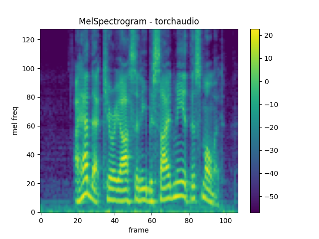
MelSpectrogram

生成梅尔频谱图涉及生成频谱图并执行梅尔刻度转换。在 torchaudio 中，MelSpectrogram 提供了此功能。

waveform, sample_rate = get_speech_sample()

n_fft = 1024
win_length = None
hop_length = 512
n_mels = 128

mel_spectrogram = T.MelSpectrogram(
    sample_rate=sample_rate,
    n_fft=n_fft,
    win_length=win_length,
    hop_length=hop_length,
    center=True,
    pad_mode="reflect",
    power=2.0,
    norm='slaney',
    onesided=True,
    n_mels=n_mels,
    mel_scale="htk",
)

melspec = mel_spectrogram(waveform)
plot_spectrogram(
    melspec[0], title="MelSpectrogram - torchaudio", ylabel='mel freq')

与librosa的对比

作为参考，以下是使用 librosa 生成梅尔尺度频谱图的等效方法。

melspec_librosa = librosa.feature.melspectrogram(
    waveform.numpy()[0],
    sr=sample_rate,
    n_fft=n_fft,
    hop_length=hop_length,
    win_length=win_length,
    center=True,
    pad_mode="reflect",
    power=2.0,
    n_mels=n_mels,
    norm='slaney',
    htk=True,
)
plot_spectrogram(
    melspec_librosa, title="MelSpectrogram - librosa", ylabel='mel freq')

mse = torch.square(melspec - melspec_librosa).mean().item()
print('Mean Square Difference: ', mse)

Out:

Mean Square Difference:  1.1827383517015733e-10

MFCC

waveform, sample_rate = get_speech_sample()

n_fft = 2048
win_length = None
hop_length = 512
n_mels = 256
n_mfcc = 256

mfcc_transform = T.MFCC(
    sample_rate=sample_rate,
    n_mfcc=n_mfcc,
    melkwargs={
      'n_fft': n_fft,
      'n_mels': n_mels,
      'hop_length': hop_length,
      'mel_scale': 'htk',
    }
)

mfcc = mfcc_transform(waveform)

plot_spectrogram(mfcc[0])

与 librosa 进行比较

melspec = librosa.feature.melspectrogram(
  y=waveform.numpy()[0], sr=sample_rate, n_fft=n_fft,
  win_length=win_length, hop_length=hop_length,
  n_mels=n_mels, htk=True, norm=None)

mfcc_librosa = librosa.feature.mfcc(
  S=librosa.core.spectrum.power_to_db(melspec),
  n_mfcc=n_mfcc, dct_type=2, norm='ortho')

plot_spectrogram(mfcc_librosa)

mse = torch.square(mfcc - mfcc_librosa).mean().item()
print('Mean Square Difference: ', mse)

Out:

Mean Square Difference:  4.261400121663428e-08

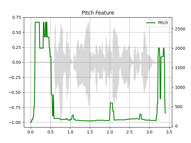
简介

waveform, sample_rate = get_speech_sample()

pitch = F.detect_pitch_frequency(waveform, sample_rate)
plot_pitch(waveform, sample_rate, pitch)
play_audio(waveform, sample_rate)

Out:

<IPython.lib.display.Audio object>

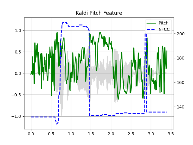
Kaldi 音高（测试版）

Kaldi Pitch 特征 [1] 是一种针对自动语音识别 (ASR) 应用进行优化的音高检测机制。这是 torchaudio 中的测试版功能，并且仅在 functional 中可用。

1. 一种针对自动语音识别优化的音高提取算法

   Ghahremani, B. BabaAli, D. Povey, K. Riedhammer, J. Trmal 和 S. Khudanpur

   2014 IEEE国际声学、语音和信号处理会议 (ICASSP), 佛罗伦萨, 2014, pp. 2494-2498, doi: 10.1109/ICASSP.2014.6854049. [摘要], [论文]

waveform, sample_rate = get_speech_sample(resample=16000)

pitch_feature = F.compute_kaldi_pitch(waveform, sample_rate)
pitch, nfcc = pitch_feature[..., 0], pitch_feature[..., 1]

plot_kaldi_pitch(waveform, sample_rate, pitch, nfcc)
play_audio(waveform, sample_rate)

Out:

<IPython.lib.display.Audio object>