介绍 || 张量 || 自动求导 || 构建模型 || TensorBoard支持 || 训练模型 || 模型理解

Pytorch深度学习框架简介

创建日期: 2021年11月30日 | 最后更新日期: 2024年1月19日 | 最后验证日期: 2024年11月5日

请跟随下方视频或在 YouTube 上观看。

PyTorch 张量

跟随视频从 03:50 开始。

首先，我们将导入 Pytorch。

import torch

让我们看看一些基本的张量操作。首先，创建张量的几种方法：

z = torch.zeros(5, 3)
print(z)
print(z.dtype)

tensor([[0., 0., 0.],
        [0., 0., 0.],
        [0., 0., 0.],
        [0., 0., 0.],
        [0., 0., 0.]])
torch.float32

上面，我们创建了一个5x3的矩阵，其中填充了零，并查询其数据类型以确定这些零是32位浮点数，这是PyTorch的默认设置。

如果你想要整数呢？你可以随时覆盖默认设置：

i = torch.ones((5, 3), dtype=torch.int16)
print(i)

tensor([[1, 1, 1],
        [1, 1, 1],
        [1, 1, 1],
        [1, 1, 1],
        [1, 1, 1]], dtype=torch.int16)

当你更改默认设置时，张量会很有帮助地在打印时报告这一点。

通常会随机初始化学习权重，常常会为PRNG指定一个特定的种子以保证结果的可重复性：

torch.manual_seed(1729)
r1 = torch.rand(2, 2)
print('A random tensor:')
print(r1)

r2 = torch.rand(2, 2)
print('\nA different random tensor:')
print(r2) # new values

torch.manual_seed(1729)
r3 = torch.rand(2, 2)
print('\nShould match r1:')
print(r3) # repeats values of r1 because of re-seed

A random tensor:
tensor([[0.3126, 0.3791],
        [0.3087, 0.0736]])

A different random tensor:
tensor([[0.4216, 0.0691],
        [0.2332, 0.4047]])

Should match r1:
tensor([[0.3126, 0.3791],
        [0.3087, 0.0736]])

PyTorch张量执行算术运算直观易懂。形状相似的张量可以相加、相乘等。与标量进行的操作会分布在张量上：

ones = torch.ones(2, 3)
print(ones)

twos = torch.ones(2, 3) * 2 # every element is multiplied by 2
print(twos)

threes = ones + twos       # addition allowed because shapes are similar
print(threes)              # tensors are added element-wise
print(threes.shape)        # this has the same dimensions as input tensors

r1 = torch.rand(2, 3)
r2 = torch.rand(3, 2)
# uncomment this line to get a runtime error
# r3 = r1 + r2

tensor([[1., 1., 1.],
        [1., 1., 1.]])
tensor([[2., 2., 2.],
        [2., 2., 2.]])
tensor([[3., 3., 3.],
        [3., 3., 3.]])
torch.Size([2, 3])

这里是一些可用的数学操作的小样本：

r = (torch.rand(2, 2) - 0.5) * 2 # values between -1 and 1
print('A random matrix, r:')
print(r)

# Common mathematical operations are supported:
print('\nAbsolute value of r:')
print(torch.abs(r))

# ...as are trigonometric functions:
print('\nInverse sine of r:')
print(torch.asin(r))

# ...and linear algebra operations like determinant and singular value decomposition
print('\nDeterminant of r:')
print(torch.det(r))
print('\nSingular value decomposition of r:')
print(torch.svd(r))

# ...and statistical and aggregate operations:
print('\nAverage and standard deviation of r:')
print(torch.std_mean(r))
print('\nMaximum value of r:')
print(torch.max(r))

A random matrix, r:
tensor([[ 0.9956, -0.2232],
        [ 0.3858, -0.6593]])

Absolute value of r:
tensor([[0.9956, 0.2232],
        [0.3858, 0.6593]])

Inverse sine of r:
tensor([[ 1.4775, -0.2251],
        [ 0.3961, -0.7199]])

Determinant of r:
tensor(-0.5703)

Singular value decomposition of r:
torch.return_types.svd(
U=tensor([[-0.8353, -0.5497],
        [-0.5497,  0.8353]]),
S=tensor([1.1793, 0.4836]),
V=tensor([[-0.8851, -0.4654],
        [ 0.4654, -0.8851]]))

Average and standard deviation of r:
(tensor(0.7217), tensor(0.1247))

Maximum value of r:
tensor(0.9956)

关于PyTorch张量的强大功能还有很多需要了解的内容， 包括如何在GPU上进行并行计算——我们会在另一段视频中详细介绍。

PyTorch 模型

跟随视频从 10:00 开始。

让我们谈谈如何在PyTorch中表达模型

import torch                     # for all things PyTorch
import torch.nn as nn            # for torch.nn.Module, the parent object for PyTorch models
import torch.nn.functional as F  # for the activation function

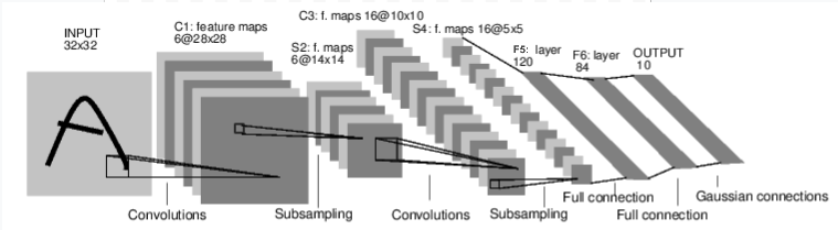
图：LeNet-5

以上是LeNet-5的示意图，它是最早期的卷积神经网络之一，也是深度学习爆炸式增长的动力之一。它被构建用于识别手写数字的小图像（MNIST数据集），并正确分类图像中代表的是哪个数字。

这是其工作原理的简化版本：

• 层 C1 是一个卷积层，意味着它会在输入图像中扫描出在训练过程中学习到的特征。它会输出一个特征图，显示在图像中它看到了每个学习到的特征的位置。这一“激活图”会在层 S2 中进行下采样。

• Layer C3 是另一个卷积层，这次扫描 C1 的激活图以寻找 特征组合。它还会输出一个描述这些特征组合的空间位置的激活图，在层 S4 中进行了下采样。

• 最后，末尾的全连接层F5、F6和OUTPUT， 是一个分类器，它将最终的激活图分类到代表10个数字中的一个的10个桶中。

我们如何用代码来表示这个简单的神经网络？

class LeNet(nn.Module):

    def __init__(self):
        super(LeNet, self).__init__()
        # 1 input image channel (black & white), 6 output channels, 5x5 square convolution
        # kernel
        self.conv1 = nn.Conv2d(1, 6, 5)
        self.conv2 = nn.Conv2d(6, 16, 5)
        # an affine operation: y = Wx + b
        self.fc1 = nn.Linear(16 * 5 * 5, 120)  # 5*5 from image dimension
        self.fc2 = nn.Linear(120, 84)
        self.fc3 = nn.Linear(84, 10)

    def forward(self, x):
        # Max pooling over a (2, 2) window
        x = F.max_pool2d(F.relu(self.conv1(x)), (2, 2))
        # If the size is a square you can only specify a single number
        x = F.max_pool2d(F.relu(self.conv2(x)), 2)
        x = x.view(-1, self.num_flat_features(x))
        x = F.relu(self.fc1(x))
        x = F.relu(self.fc2(x))
        x = self.fc3(x)
        return x

    def num_flat_features(self, x):
        size = x.size()[1:]  # all dimensions except the batch dimension
        num_features = 1
        for s in size:
            num_features *= s
        return num_features

查看这段代码，你应该能够发现它与上面的图表有一些结构上的相似之处。

这展示了典型的PyTorch模型的结构：

• 它继承自 torch.nn.Module - 模块可以嵌套 - 实际上， 甚至 Conv2d 和 Linear 层类也继承自 torch.nn.Module.

• 一个模型将有一个__init__()函数，其中它实例化其层，并加载任何可能需要的数据 artifact（例如，一个 NLP 模型可能会加载词汇表）。

• 一个模型将有一个forward()函数。这就是实际计算发生的地方：输入通过网络层和各种函数生成输出。

• 除了这一点之外，你可以像其他任何 Python 类一样构建你的模型类，添加你需要的支持模型计算的属性和方法。

让我们实例化这个对象，并通过一个样本输入运行一下。

net = LeNet()
print(net)                         # what does the object tell us about itself?

input = torch.rand(1, 1, 32, 32)   # stand-in for a 32x32 black & white image
print('\nImage batch shape:')
print(input.shape)

output = net(input)                # we don't call forward() directly
print('\nRaw output:')
print(output)
print(output.shape)

LeNet(
  (conv1): Conv2d(1, 6, kernel_size=(5, 5), stride=(1, 1))
  (conv2): Conv2d(6, 16, kernel_size=(5, 5), stride=(1, 1))
  (fc1): Linear(in_features=400, out_features=120, bias=True)
  (fc2): Linear(in_features=120, out_features=84, bias=True)
  (fc3): Linear(in_features=84, out_features=10, bias=True)
)

Image batch shape:
torch.Size([1, 1, 32, 32])

Raw output:
tensor([[ 0.0898,  0.0318,  0.1485,  0.0301, -0.0085, -0.1135, -0.0296,  0.0164,
          0.0039,  0.0616]], grad_fn=<AddmmBackward0>)
torch.Size([1, 10])

以上有一些重要的事情正在发生：

首先，我们实例化LeNet类，并打印net 对象。torch.nn.Module的子类会报告它创建的层及其形状和参数。这可以在您想要了解其处理流程概要时提供一个方便的概述。

在那之下，我们创建了一个代表32x32像素单色图像的假输入。通常情况下，你会加载一个图像块并将其转换为这种形状的张量。

您可能已经注意到我们的张量多了一维——批量维度。PyTorch模型假设它们正在处理数据的批量——例如，16张我们图像瓦片的批量具有形状(16, 1, 32, 32)。由于我们只使用一张图像，因此我们创建一个形状为(1, 1, 32, 32)的批量。

我们通过像调用函数一样调用模型来进行推理： net(input)。这次调用的输出代表了模型对输入表示某个特定数字的信心程度。（由于这个模型还没有学习任何东西，我们不应该期望在输出中看到任何信号。）查看output的形状，我们可以发现它也有一个批次维度，其大小应该始终与输入批次维度的大小匹配。如果我们传入的是16个实例的输入批次，output的形状将会是(16, 10)。

数据集和数据加载器

跟随视频从 14:00 开始。

下面，我们将演示如何使用 TorchVision 中提供的一种可下载且开放访问的数据集，对图像进行转换以便供您的模型使用，并如何使用 DataLoader 向您的模型喂送数据批次。

我们需要首先将传入的图像转换为一个 PyTorch 张量。

#%matplotlib inline

import torch
import torchvision
import torchvision.transforms as transforms

transform = transforms.Compose(
    [transforms.ToTensor(),
     transforms.Normalize((0.4914, 0.4822, 0.4465), (0.2470, 0.2435, 0.2616))])

在这里，我们为输入指定了两种变换：

• transforms.ToTensor() 将由Pillow加载的图像转换为 PyTorch张量。

• transforms.Normalize() 调整张量的值，使其平均值为零且标准差为1.0。大多数激活函数在x = 0附近梯度最强，因此将数据集中在该处可以加快学习速度。 传递给变换的值是数据集中图像的rgb值的均值（第一个元组）和标准差（第二个元组）。您可以自己运行这几行代码来计算这些值：

  ```

  from torch.utils.data import ConcatDataset transform = transforms.Compose([transforms.ToTensor()]) trainset = torchvision.datasets.CIFAR10(root=’./data’, train=True,

  download=True, transform=transform)

  #stack all train images together into a tensor of shape #(50000, 3, 32, 32) x = torch.stack([sample[0] for sample in ConcatDataset([trainset])])

  #get the mean of each channel mean = torch.mean(x, dim=(0,2,3)) #tensor([0.4914, 0.4822, 0.4465]) std = torch.std(x, dim=(0,2,3)) #tensor([0.2470, 0.2435, 0.2616])

  ```

还有许多其他变换可供选择，包括裁剪、居中、旋转和反射。

接下来，我们将创建一个CIFAR10数据集的实例。这是一个包含32x32颜色图像的小瓦片集合，代表10类对象：其中6类是动物（torio、猫、鹿、狗、青蛙、马），另外4类是车辆（飞机、汽车、船、卡车）：

trainset = torchvision.datasets.CIFAR10(root='./data', train=True,
                                        download=True, transform=transform)

Downloading https://www.cs.toronto.edu/~kriz/cifar-10-python.tar.gz to ./data/cifar-10-python.tar.gz

  0%|          | 0.00/170M [00:00<?, ?B/s]
  0%|          | 655k/170M [00:00<00:25, 6.55MB/s]
  4%|4         | 7.41M/170M [00:00<00:03, 42.4MB/s]
 11%|#1        | 19.1M/170M [00:00<00:01, 76.4MB/s]
 18%|#7        | 30.3M/170M [00:00<00:01, 90.5MB/s]
 23%|##3       | 39.6M/170M [00:00<00:01, 91.2MB/s]
 30%|###       | 51.3M/170M [00:00<00:01, 100MB/s]
 36%|###5      | 61.4M/170M [00:00<00:01, 98.8MB/s]
 42%|####2     | 72.3M/170M [00:00<00:00, 102MB/s]
 49%|####8     | 83.2M/170M [00:00<00:00, 104MB/s]
 55%|#####4    | 93.6M/170M [00:01<00:00, 102MB/s]
 62%|######1   | 105M/170M [00:01<00:00, 106MB/s]
 68%|######7   | 116M/170M [00:01<00:00, 103MB/s]
 74%|#######4  | 127M/170M [00:01<00:00, 104MB/s]
 81%|########  | 138M/170M [00:01<00:00, 107MB/s]
 87%|########7 | 149M/170M [00:01<00:00, 106MB/s]
 94%|#########3| 160M/170M [00:01<00:00, 108MB/s]
100%|##########| 170M/170M [00:01<00:00, 98.3MB/s]
Extracting ./data/cifar-10-python.tar.gz to ./data

注意

当你运行上面的单元格时，可能会花费一些时间下载数据集。

这是一名在PyTorch中创建数据集对象的示例。可下载的数据集（如上面的CIFAR-10）是torch.utils.data.Dataset的子类。Dataset类包括在TorchVision、Torchtext和TorchAudio中的可下载数据集，以及torchvision.datasets.ImageFolder这样的实用数据集类，它可以读取带有标签的图片文件夹。您也可以创建自己的Dataset的子类。

当我们实例化我们的数据集时，需要告诉它一些信息：

• 我们希望数据存储的文件系统路径。

• 无论我们是否使用这个数据集进行训练；大多数数据集都会被划分为训练集和测试集。

• 如果我们还没有下载数据集，是否希望现在下载。

• 我们想要应用于数据的转换。

一旦您的数据集准备就绪，您可以将其提供给DataLoader：

trainloader = torch.utils.data.DataLoader(trainset, batch_size=4,
                                          shuffle=True, num_workers=2)

一个 Dataset 子类封装了对数据的访问，并针对其提供的数据类型进行了专门化。DataLoader 对数据一无所知，但它会根据你指定的参数将 Dataset 提供的输入张量组织成批次。

在上面的例子中，我们请求了一个DataLoader从trainset中随机化顺序地（shuffle=True）提供每批4张图像，并告诉它启动两个工人从磁盘加载数据。

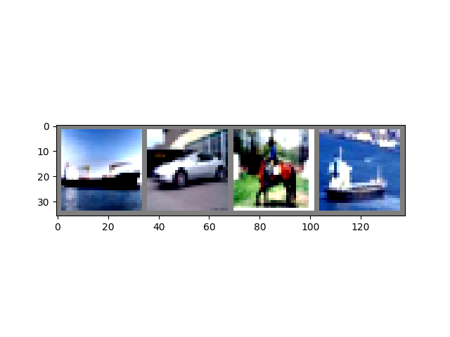
可视化 DataLoader 服务的批次是一个好习惯：

import matplotlib.pyplot as plt
import numpy as np

classes = ('plane', 'car', 'bird', 'cat',
           'deer', 'dog', 'frog', 'horse', 'ship', 'truck')

def imshow(img):
    img = img / 2 + 0.5     # unnormalize
    npimg = img.numpy()
    plt.imshow(np.transpose(npimg, (1, 2, 0)))


# get some random training images
dataiter = iter(trainloader)
images, labels = next(dataiter)

# show images
imshow(torchvision.utils.make_grid(images))
# print labels
print(' '.join('%5s' % classes[labels[j]] for j in range(4)))

Clipping input data to the valid range for imshow with RGB data ([0..1] for floats or [0..255] for integers). Got range [-0.49473685..1.5632443].
 ship   car horse  ship

运行上面的单元格应该会显示四张图片组成的条带，并且每张图片正确的标签。

训练您的PyTorch模型

跟随视频从 17:10 开始。

让我们把所有拼图组合在一起，并训练一个模型：

#%matplotlib inline

import torch
import torch.nn as nn
import torch.nn.functional as F
import torch.optim as optim

import torchvision
import torchvision.transforms as transforms

import matplotlib
import matplotlib.pyplot as plt
import numpy as np

首先，我们需要训练集和测试集。如果你还没有下载，请运行下方的单元格以确保数据集已经下载。（这可能需要一分钟时间）

transform = transforms.Compose(
    [transforms.ToTensor(),
     transforms.Normalize((0.5, 0.5, 0.5), (0.5, 0.5, 0.5))])

trainset = torchvision.datasets.CIFAR10(root='./data', train=True,
                                        download=True, transform=transform)
trainloader = torch.utils.data.DataLoader(trainset, batch_size=4,
                                          shuffle=True, num_workers=2)

testset = torchvision.datasets.CIFAR10(root='./data', train=False,
                                       download=True, transform=transform)
testloader = torch.utils.data.DataLoader(testset, batch_size=4,
                                         shuffle=False, num_workers=2)

classes = ('plane', 'car', 'bird', 'cat',
           'deer', 'dog', 'frog', 'horse', 'ship', 'truck')

Files already downloaded and verified
Files already downloaded and verified

我们将会检查来自 DataLoader 的输出：

import matplotlib.pyplot as plt
import numpy as np

# functions to show an image


def imshow(img):
    img = img / 2 + 0.5     # unnormalize
    npimg = img.numpy()
    plt.imshow(np.transpose(npimg, (1, 2, 0)))


# get some random training images
dataiter = iter(trainloader)
images, labels = next(dataiter)

# show images
imshow(torchvision.utils.make_grid(images))
# print labels
print(' '.join('%5s' % classes[labels[j]] for j in range(4)))

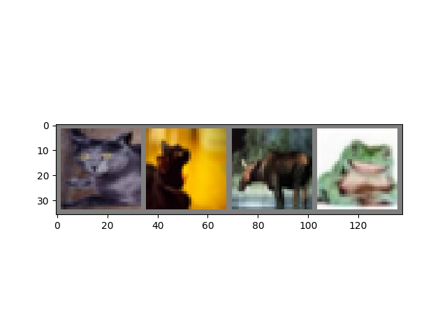
cat   cat  deer  frog

这是我们将在其中进行训练的模型。如果看起来很熟悉，那是因为它是一种早期视频中讨论过的LeNet变体，适应了三色图像。

class Net(nn.Module):
    def __init__(self):
        super(Net, self).__init__()
        self.conv1 = nn.Conv2d(3, 6, 5)
        self.pool = nn.MaxPool2d(2, 2)
        self.conv2 = nn.Conv2d(6, 16, 5)
        self.fc1 = nn.Linear(16 * 5 * 5, 120)
        self.fc2 = nn.Linear(120, 84)
        self.fc3 = nn.Linear(84, 10)

    def forward(self, x):
        x = self.pool(F.relu(self.conv1(x)))
        x = self.pool(F.relu(self.conv2(x)))
        x = x.view(-1, 16 * 5 * 5)
        x = F.relu(self.fc1(x))
        x = F.relu(self.fc2(x))
        x = self.fc3(x)
        return x


net = Net()

我们需要的最后一部分是损失函数和优化器：

criterion = nn.CrossEntropyLoss()
optimizer = optim.SGD(net.parameters(), lr=0.001, momentum=0.9)

如本视频早先所述，损失函数衡量的是模型预测值与我们理想输出之间的差距。交叉熵损失函数是我们这类分类模型中常用的损失函数。

优化器是驱动学习的动力。这里我们创建了一个实现随机梯度下降的优化器，这是一种较为直观的优化算法。除了算法参数，比如学习率(lr)和动量外，我们还传入了net.parameters()，这是一个包含模型中所有学习权重的集合——优化器会调整这些权重。

最后，这一切都会被组装进训练循环中。请运行这个单元格，因为它执行起来可能需要几分钟时间。

for epoch in range(2):  # loop over the dataset multiple times

    running_loss = 0.0
    for i, data in enumerate(trainloader, 0):
        # get the inputs
        inputs, labels = data

        # zero the parameter gradients
        optimizer.zero_grad()

        # forward + backward + optimize
        outputs = net(inputs)
        loss = criterion(outputs, labels)
        loss.backward()
        optimizer.step()

        # print statistics
        running_loss += loss.item()
        if i % 2000 == 1999:    # print every 2000 mini-batches
            print('[%d, %5d] loss: %.3f' %
                  (epoch + 1, i + 1, running_loss / 2000))
            running_loss = 0.0

print('Finished Training')

[1,  2000] loss: 2.195
[1,  4000] loss: 1.876
[1,  6000] loss: 1.655
[1,  8000] loss: 1.576
[1, 10000] loss: 1.519
[1, 12000] loss: 1.466
[2,  2000] loss: 1.421
[2,  4000] loss: 1.376
[2,  6000] loss: 1.336
[2,  8000] loss: 1.335
[2, 10000] loss: 1.326
[2, 12000] loss: 1.270
Finished Training

在这里，我们只进行了 2个训练周期（第1行）——也就是说，对训练数据集进行了两次遍历。每次遍历都有一个内部循环（第4行），用于遍历训练数据，提供经过转换的输入图像及其正确的标签。

清零梯度（第9行）是一个重要的步骤。梯度会在一批数据上累积；如果我们不为每一批数据重置它们，梯度将会持续累积，这将提供错误的梯度值，使得学习变得不可能。

在第12行，我们请求模型对这个批次进行预测。在接下来的行（第13行），我们计算损失 - 模型预测与正确输出之间的差异。outputs（模型预测）和labels（正确输出）。

在第14行，我们进行一次 backward() 轮计算，并计算出将引导学习的梯度。

在第15行，优化器执行一次学习步骤 - 它使用来自backward()调用的梯度来调整学习权重，以减少损失。

循环的其余部分会进行一些轻量级的报告，包括当前的epoch编号、已完成的训练实例数量以及训练循环中收集到的损失值。

当你运行上面的单元格时,你应该会看到类似这样的内容：

[1,  2000] loss: 2.235
[1,  4000] loss: 1.940
[1,  6000] loss: 1.713
[1,  8000] loss: 1.573
[1, 10000] loss: 1.507
[1, 12000] loss: 1.442
[2,  2000] loss: 1.378
[2,  4000] loss: 1.364
[2,  6000] loss: 1.349
[2,  8000] loss: 1.319
[2, 10000] loss: 1.284
[2, 12000] loss: 1.267
Finished Training

请注意，损失值呈现单调下降趋势，表明我们的模型正在持续提高在训练数据集上的性能。

作为最后一步，我们应该检查模型是否实际上在进行 泛化 学习，而不是简单地“记忆”数据集。这被称为 过拟合，通常表明数据集太小（没有足够的例子进行泛化学习），或者模型的学习参数过多，超过了正确建模数据集所需的数量。

这是将数据集分为训练集和测试集的原因——为了测试模型的通用性，我们让它对未参与训练的数据进行预测：

correct = 0
total = 0
with torch.no_grad():
    for data in testloader:
        images, labels = data
        outputs = net(images)
        _, predicted = torch.max(outputs.data, 1)
        total += labels.size(0)
        correct += (predicted == labels).sum().item()

print('Accuracy of the network on the 10000 test images: %d %%' % (
    100 * correct / total))

Accuracy of the network on the 10000 test images: 54 %

如果你跟着操作了，到目前为止你应该会看到模型的准确率大约为50%。这并不完全是最先进的水平，但远远超过了我们从随机输出中期望的10%准确率。这表明模型在一定程度上确实学到了一些通用的知识。